FFT plots – Programming

The role of this notebook is to demonstrate how to make easy-to-read ticks on a loglog FFT plot

import numpy as np
import matplotlib.pyplot as plt

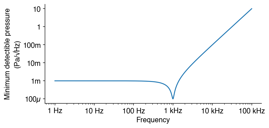
In this notebook, we will generate some sample FFT by looking at the inverse scaling of damped harmonic oscillator. This is something a buddy of mine worked on in graduate school for measuring pressure. The minimum detectible pressure that he could measure was inversely related to the harmonic oscillator response

def H(f, f0, zeta):
    """The frequency response of a damped harmonic oscillator
    
    f: The range of frequencies to plot
    f0: Center frequency
    zeta: The damping ratio
    """
    return ((1 - (f/f0)**2)**2 + (2*zeta*f/f0)**2)**(-.5)

Next, compute the minimum detectible pressure in units of Pascal/sqrt(Hz)

f0 = 1e3 # 1 kHz
zeta = .05
freqs = np.logspace(0, 5, 2000)
y0 = 1e-3
hs = H(freqs, f0, zeta)
mdp = y0 / hs # Minimum detectible pressure

Here is the code that you want to copy in for quickly looking up SI prefixes

from math import floor
SI_PREFIXES = 'qryzafpnµm1kMGTPEZYRQ'
import matplotlib.ticker as mticks

def fmt_freq(v, _): # Format frequency axis
    frac_exponent_over_3 = floor(np.log10(v) / 3)
    idx_prefix = 10 + frac_exponent_over_3
    prefix = SI_PREFIXES[idx_prefix]
    if prefix == '1': prefix = ''
    return f'{v/(1000**frac_exponent_over_3):.0f} {prefix}Hz'

def fmt_y(v, _): # Format y axis
    frac_exponent_over_3 = floor(np.log10(v) / 3)
    idx_prefix = 10 + frac_exponent_over_3
    prefix = SI_PREFIXES[idx_prefix]
    if prefix == '1': prefix = ''
    return f'{v/(1000**frac_exponent_over_3):.0f}{prefix}'

fig, ax = plt.subplots()
ax.loglog(freqs, y0/hs)

ax.set_ylabel('Minimum detectible pressure\n(Pa/√Hz)')
ax.set_xlabel('Frequency')
ax.xaxis.set_major_formatter(fmt_freq)
ax.yaxis.set_major_formatter(fmt_y)
ax.yaxis.set_major_locator(mticks.LogLocator(base=10, numticks=100)) # Make sure you don't skip decades